Reporting with tidylearn • tidylearn

Overview

tidylearn is designed so that analysis results flow directly into reports. Every model produces tidy tibbles, ggplot2 visualisations, and — with the tl_table_*() functions — formatted gt tables, all with a consistent interface. This vignette walks through the reporting tools available.

library(tidylearn)
library(dplyr)
library(ggplot2)
library(gt)

Plots

tidylearn’s plot() method dispatches to the right visualisation for each model type. All plots are ggplot2 objects — themeable, composable, and convertible to plotly.

Regression

model_reg <- tl_model(mtcars, mpg ~ wt + hp, method = "linear")

# Actual vs predicted — one call
plot(model_reg, type = "actual_predicted")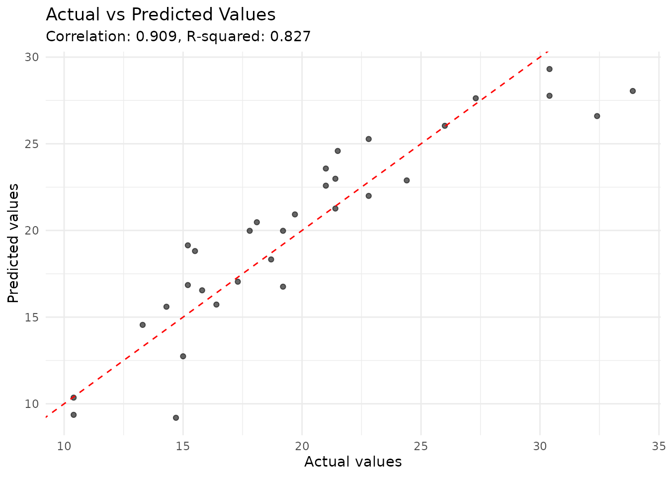

Classification

split <- tl_split(iris, prop = 0.7, stratify = "Species", seed = 42)
model_clf <- tl_model(split$train, Species ~ ., method = "forest")

plot(model_clf, type = "confusion")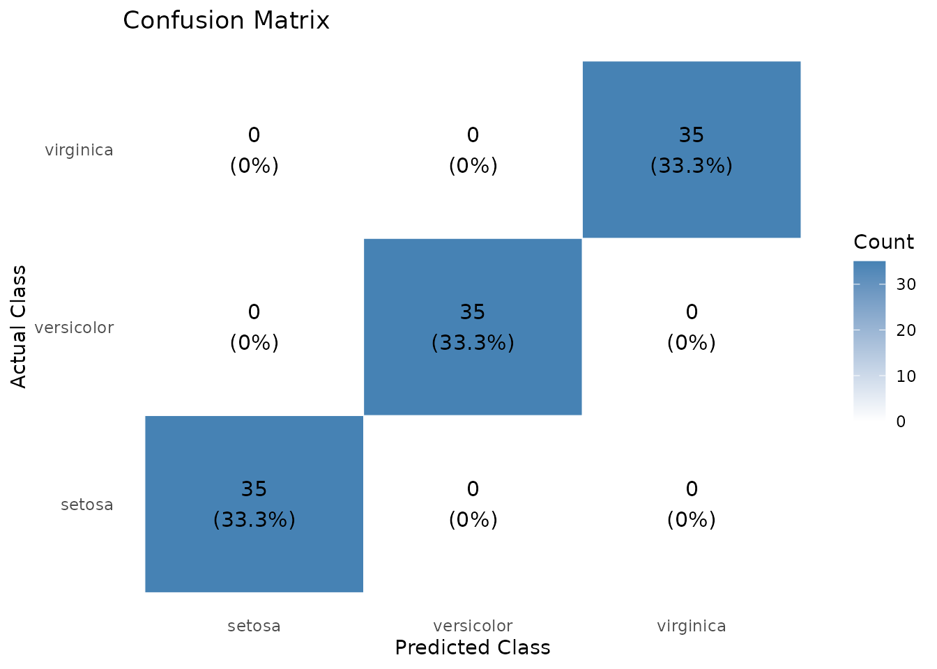

PCA

pca <- tidy_pca(USArrests, scale = TRUE)

tidy_pca_screeplot(pca)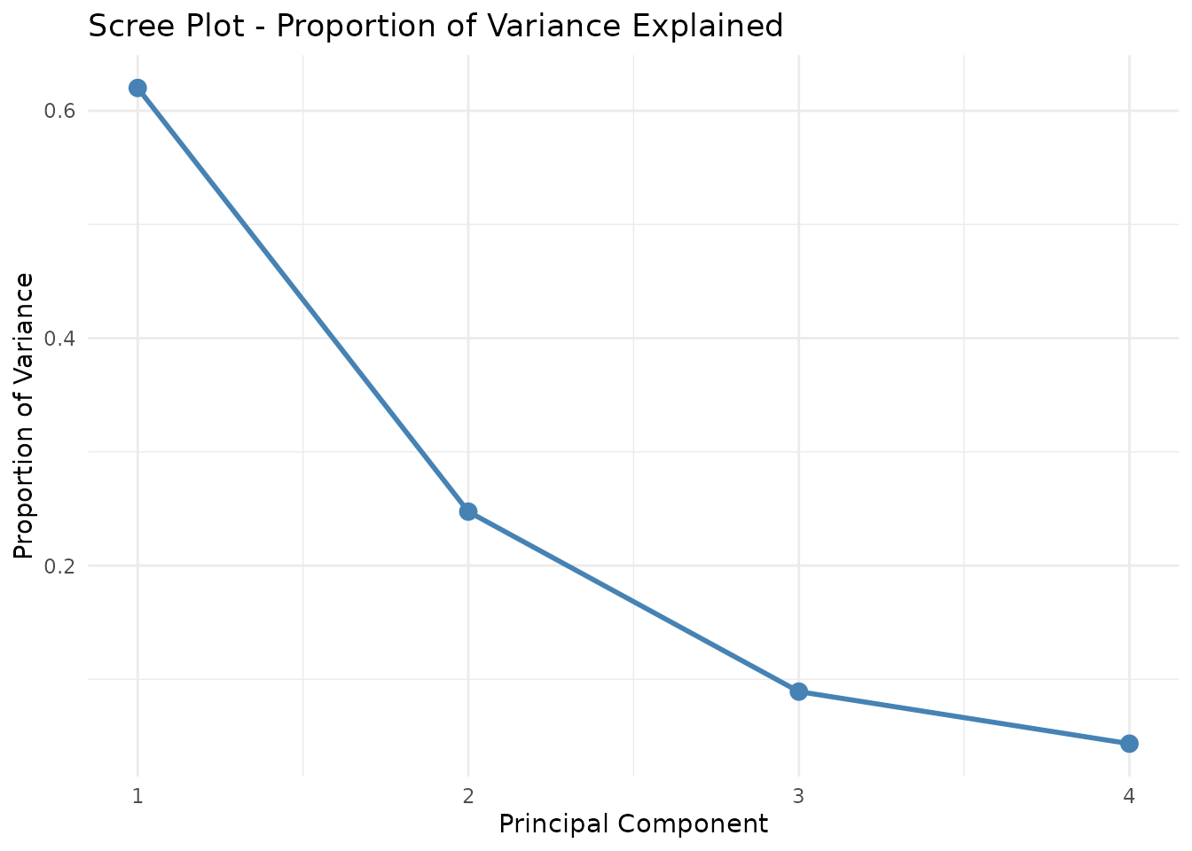

tidy_pca_biplot(pca, label_obs = TRUE)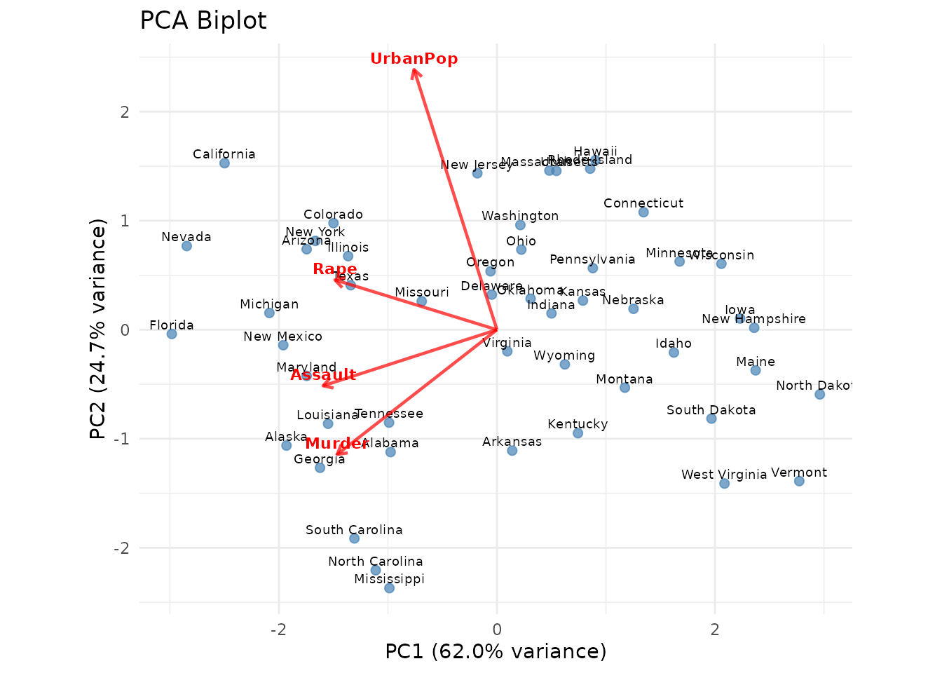

Regularisation

model_lasso <- tl_model(mtcars, mpg ~ ., method = "lasso")

tl_plot_regularization_path(model_lasso)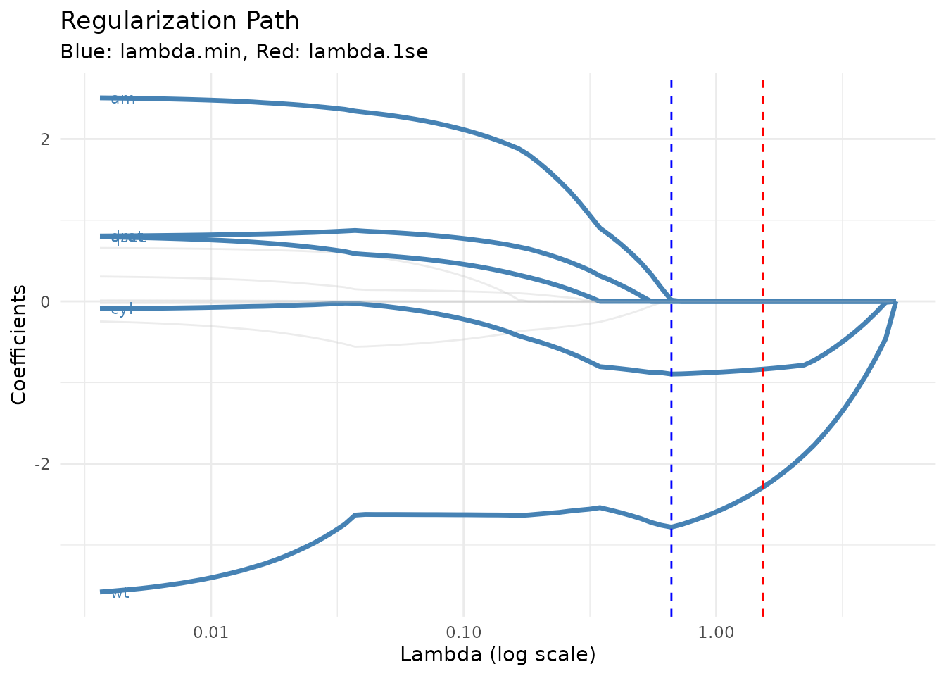

tl_plot_regularization_cv(model_lasso)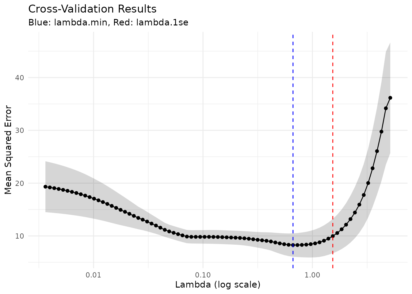

Tables

The tl_table() family mirrors the plot interface but produces formatted gt tables instead. Like plot(), tl_table() dispatches based on model type and a type parameter:

tl_table(model)                       # auto-selects the best table type
tl_table(model, type = "coefficients") # specific type

Evaluation Metrics

tl_table_metrics(model_reg)

Metric	Value
Model Evaluation Metrics
Rmse	2.4689
Mae	1.9015
Rsq	0.8268
tidylearn \| linear (regression) \| mpg ~ wt + hp \| n = 32

Coefficients

For linear and logistic models, the table includes standard errors, test statistics, and p-values, with significant terms highlighted:

tl_table_coefficients(model_reg)

Term	Estimate	Std. Error	t value	p
Linear Model Coefficients
(Intercept)	37.2273	1.5988	23.2847	2.57 × 10⁻²⁰	*
wt	−3.8778	0.6327	−6.1287	1.12 × 10⁻⁶	*
hp	−0.0318	0.0090	−3.5187	1.45 × 10⁻³	*
tidylearn \| linear (regression) \| mpg ~ wt + hp \| n = 32

For regularised models, coefficients are sorted by magnitude and zero coefficients are greyed out:

tl_table_coefficients(model_lasso)

Term	Coefficient	\|Coefficient\|
Lasso Coefficients
lambda = 1.536 (1se)
(Intercept)	33.4721	33.4721
wt	−2.2863	2.2863
cyl	−0.8339	0.8339
hp	−0.0059	0.0059
disp	0.0000	0.0000
drat	0.0000	0.0000
qsec	0.0000	0.0000
vs	0.0000	0.0000
am	0.0000	0.0000
gear	0.0000	0.0000
carb	0.0000	0.0000
tidylearn \| lasso (regression) \| mpg ~ . \| n = 32

Confusion Matrix

A formatted confusion matrix with correct predictions highlighted on the diagonal:

tl_table_confusion(model_clf, new_data = split$test)

Actual	Predicted
Confusion Matrix
Actual	setosa	versicolor	virginica
setosa	15	0	0
versicolor	0	14	1
virginica	0	2	13
tidylearn \| forest (classification) \| Species ~ . \| n = 105

Feature Importance

A ranked importance table with a colour gradient:

tl_table_importance(model_clf)

Feature	Importance
Feature Importance
Top 4 features
Petal.Length	100.00
Petal.Width	93.33
Sepal.Length	27.43
Sepal.Width	10.52
tidylearn \| forest (classification) \| Species ~ . \| n = 105

PCA Variance Explained

Cumulative variance is coloured green to highlight how many components are needed:

pca_model <- tl_model(USArrests, method = "pca")
tl_table_variance(pca_model)

Component	Std. Dev.	Variance	Proportion	Cumulative
PCA Variance Explained
PC1	1.5749	2.4802	62.0%	62.0%
PC2	0.9949	0.9898	24.7%	86.8%
PC3	0.5971	0.3566	8.9%	95.7%
PC4	0.4164	0.1734	4.3%	100.0%
tidylearn \| pca \| n = 50

PCA Loadings

A diverging red–blue colour scale highlights strong positive and negative loadings:

tl_table_loadings(pca_model)

Variable	PC1	PC2	PC3	PC4
PCA Loadings
Murder	−0.536	−0.418	0.341	0.649
Assault	−0.583	−0.188	0.268	−0.743
UrbanPop	−0.278	0.873	0.378	0.134
Rape	−0.543	0.167	−0.818	0.089
tidylearn \| pca \| n = 50

Cluster Summary

Cluster sizes and mean feature values:

km <- tl_model(iris[, 1:4], method = "kmeans", k = 3)
tl_table_clusters(km)

Cluster	Size	Sepal.Length	Sepal.Width	Petal.Length	Petal.Width
Cluster Summary
kmeans \| 3 clusters
1	50	5.01	3.43	1.46	0.25
2	38	6.85	3.07	5.74	2.07
3	62	5.90	2.75	4.39	1.43
tidylearn \| kmeans \| n = 150

Model Comparison

Compare multiple models side-by-side:

m1 <- tl_model(split$train, Species ~ ., method = "svm")
m2 <- tl_model(split$train, Species ~ ., method = "forest")
m3 <- tl_model(split$train, Species ~ ., method = "tree")

tl_table_comparison(
  m1, m2, m3,
  new_data = split$test,
  names = c("SVM", "Random Forest", "Decision Tree")
)

Metric	SVM	Random Forest	Decision Tree
Model Comparison
3 models compared
Accuracy	0.9111	0.9333	0.8889
tidylearn \| n = 45

Interactive Reporting with plotly

Because all plot functions return ggplot2 objects, converting to interactive plotly charts is a one-liner:

library(plotly)

ggplotly(plot(model_reg, type = "actual_predicted"))
ggplotly(tidy_pca_biplot(pca, label_obs = TRUE))
ggplotly(tl_plot_regularization_path(model_lasso))

Putting It Together

A typical reporting workflow combines plots and tables for the same model. Because the interface is consistent, the same pattern works regardless of the algorithm:

# Fit
model <- tl_model(split$train, Species ~ ., method = "forest")

# Evaluate
tl_table_metrics(model, new_data = split$test)

Metric	Value
Model Evaluation Metrics
Accuracy	0.9333
tidylearn \| forest (classification) \| Species ~ . \| n = 105


# Visualise
plot(model, type = "confusion")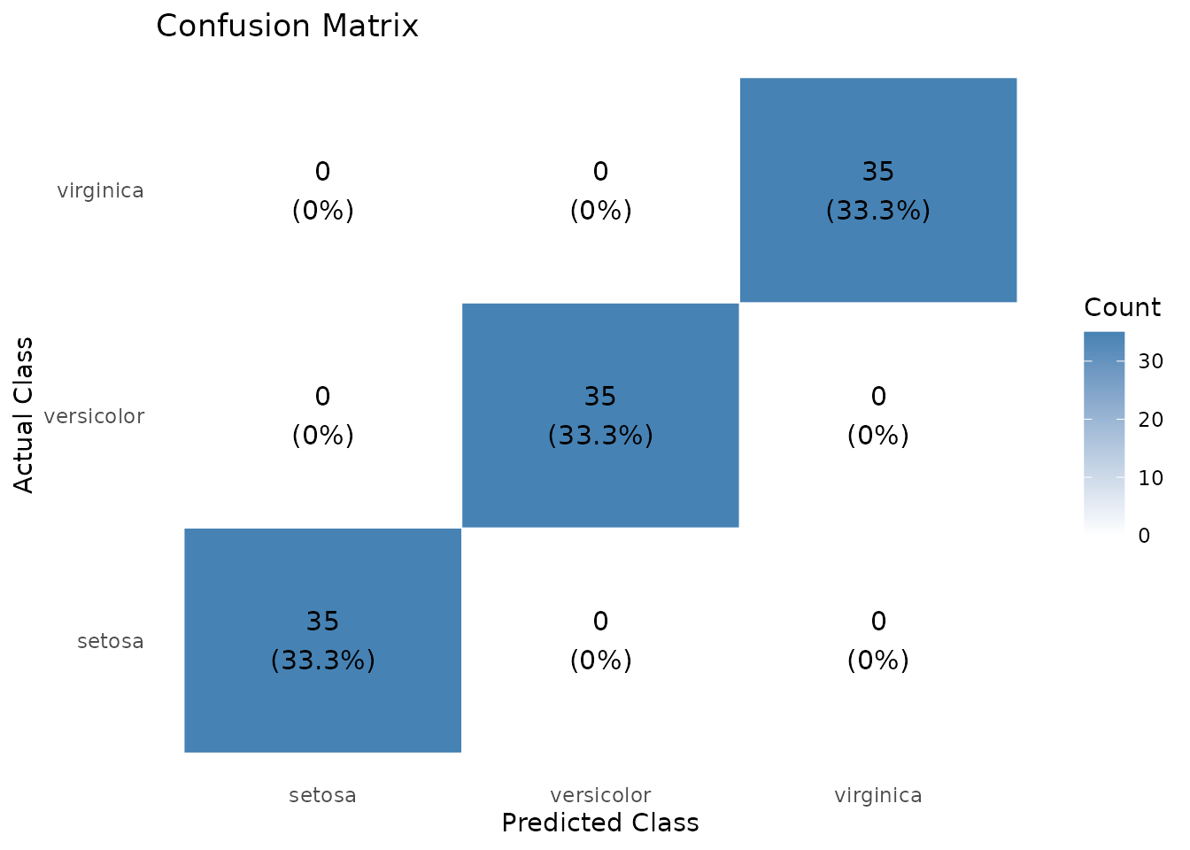


# Drill into feature importance
tl_table_importance(model, top_n = 4)

Feature	Importance
Feature Importance
Top 4 features
Petal.Length	100.00
Petal.Width	99.13
Sepal.Length	32.47
Sepal.Width	13.13
tidylearn \| forest (classification) \| Species ~ . \| n = 105

Swap method = "forest" for method = "tree" or method = "svm" and the reporting code above works without modification.